5. High Order Taylor Maps II

(original by Dario Izzo - extended by Ekin Ozturk)

Building upon the notebook here, we show the use of desolver for numerically integrating the system of differential equations \(\dot{\mathbf y} = \mathbf f(\mathbf y)\):

\[\begin{split}\begin{array}{l} \dot r = v_r \\ \dot v_r = - \frac 1{r^2} + r v_\theta^2\\ \dot \theta = v_\theta \\ \dot v_\theta = -2 \frac{v_\theta v_r}{r} + T \end{array}\end{split}\]

which describe, in non dimensional units, the motion of a mass point object around some primary body perturbed by a fixed thrust \(T\) acting in the direction perpendicular to the radius vector. We show how we can build a high order Taylor map (HOTM, indicated with \(\mathcal M\)) representing the final state of the system at the time \(T\) as a function of the initial conditions.

In other words, we build a polinomial representation of the relation \(\mathbf y(T) = \mathbf f(\mathbf y(0), T)\). Writing the initial conditions as \(\mathbf y(0) = \overline {\mathbf y}(0) + \mathbf {dy}\), our HOTM will be written as:

\[\mathbf y(T) = \mathcal M(\mathbf {dy})\]

and will be valid in a neighbourhood of \(\overline {\mathbf y}(0)\).

5.1. Importing Stuff

%matplotlib inline
from matplotlib import pyplot as plt

import os
import numpy as np

os.environ['DES_BACKEND'] = 'numpy'
import desolver as de
import desolver.backend as D
from desolver.backend import gdual_double as gdual

PyAudi backend is available.
Using numpy backend

T = 1e-3

@de.rhs_prettifier(equ_repr="[vr, -1/r**2 + r*vt**2, vt, -2*vt*vr/r]", md_repr=r"""$$
\begin{array}{l}
\dot r = v_r \\
\dot v_r = - \frac 1{r^2} + r v_\theta^2\\
\dot \theta = v_\theta \\
\dot v_\theta = -2 \frac{v_\theta v_r}{r}
\end{array}
$$""")
def eom_kep_polar(t,y,**kwargs):
    return D.array([y[1], - 1 / y[0] / y[0] + y[0] * y[3]*y[3], y[3], -2*y[3]*y[1]/y[0] - T])

eom_kep_polar

\[\begin{split}\begin{array}{l} \dot r = v_r \\ \dot v_r = - \frac 1{r^2} + r v_\theta^2\\ \dot \theta = v_\theta \\ \dot v_\theta = -2 \frac{v_\theta v_r}{r} \end{array}\end{split}\]

# The initial conditions
ic = [1.,0.1,0.,-1.]

5.2. We perform the numerical integration using floats (the standard way)

D.set_float_fmt('float64')
float_integration = de.OdeSystem(eom_kep_polar, y0=ic, dense_output=False, t=(0, 300.), dt=0.01, rtol=1e-10, atol=1e-10, constants=dict())

float_integration.set_method("RK45")
float_integration.integrate(eta=True)

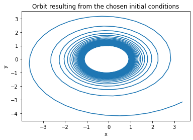
# Here we transform from polar to cartesian coordinates
# to then plot
y = float_integration.y
cx = [it[0]*np.sin(it[2]) for it in y.astype(np.float64)]
cy = [it[0]*np.cos(it[2]) for it in y.astype(np.float64)]
plt.plot(cx,cy)
plt.title("Orbit resulting from the chosen initial conditions")
plt.xlabel("x")
plt.ylabel("y")

Text(0, 0.5, 'y')

5.3. We perform the numerical integration using gduals (to get a HOTM)

# Order of the Taylor Map. If we have 4 variables the number of terms in the Taylor expansion in 329  at order 7
order = 6
# We now define the initial conditions as gdual (not float)
ic_g = [gdual(ic[0], "r", order), gdual(ic[1], "vr", order), gdual(ic[2], "t", order), gdual(ic[3], "vt", order)]

import time
start_time = time.time()
D.set_float_fmt('gdual_double')
gdual_integration = de.OdeSystem(eom_kep_polar, y0=ic_g, dense_output=False, t=(0, 300.), dt=0.01, rtol=1e-10, atol=1e-10, constants=dict())

gdual_integration.set_method("RK45")
gdual_integration.integrate(eta=True)
print("--- %s seconds ---" % (time.time() - start_time))

--- 38.72461462020874 seconds ---

# We extract the last point
yf = gdual_integration.y[-1]
# And unpack it into some convinient names
rf,vrf,tf,vtf = yf
# We compute the final cartesian components
xf = rf * D.sin(tf)
yf = rf * D.cos(tf)
# Note that you can get the latex representation of the gdual
print(xf._repr_latex_())
print("xf (latex):")
xf

\[ 5.27792e+09{dvr}^{2}{dvt}^{2}+2.38683e+07{dr}{dt}{dvr}^{2}+812955{dr}{dt}^{3}{dvt}+0.528723{dt}^{3}-3.96318e+08{dvr}^{3}{dvt}-4.87979e+09{dr}^{2}{dt}{dvt}-1.17038e+16{dr}{dvr}{dvt}^{4}-0.00467575{dt}^{6}+6.75558e+13{dr}{dvr}{dvt}^{3}+1.41974e+12{dr}^{3}{dt}^{2}{dvt}+1.05585e+10{dr}{dt}^{2}{dvr}^{2}{dvt}-4.74308e+17{dr}^{4}{dvt}^{2}-1.9878e+15{dvt}^{6}+1.7157e+13{dr}^{2}{dvr}^{2}{dvt}-2.09573e+12{dr}^{2}{dt}{dvt}^{2}+1.43888e+15{dr}^{4}{dvt}+2.20856e+09{dr}{dvt}^{2}+2.75642e+06{dr}^{2}{dt}^{2}-1.97312e+11{dr}{dt}{dvr}{dvt}^{2}-5.40989e+08{dr}^{3}{dt}^{3}+1.03991e+08{dvr}{dvt}^{2}-1.91427e+07{dt}^{3}{dvr}{dvt}^{2}+3.36654-1.92511e+13{dr}^{2}{dvr}^{4}+689698{dt}^{2}{dvt}^{2}-4.07038e+08{dr}{dt}^{3}{dvt}^{2}-3.93014e+09{dvr}^{6}-6200.56{dr}{dt}-8.73108e+10{dt}{dvt}^{4}+1.43057e+12{dvr}^{2}{dvt}^{3}+4.59063e+08{dr}^{2}{dt}{dvr}-230.032{dr}{dt}^{4}+7.92742e+08{dr}{dvr}^{3}-8.57426e+12{dr}{dvr}^{2}{dvt}^{2}-2.63896e+09{dt}^{2}{dvr}^{2}{dvt}^{2}-93896{dt}^{2}{dvr}^{3}+1.16891e+15{dvr}{dvt}^{5}+2.01684e+11{dr}^{2}{dt}^{2}{dvr}{dvt}-1.34155e+11{dr}^{3}{dt}^{2}{dvr}+2.70709e+14{dr}^{3}{dvr}{dvt}-7.0871e+11{dr}^{2}{dt}{dvr}^{3}-518252{dr}{dvr}-1.19378e+17{dr}^{2}{dvt}^{4}+6.98014e+11{dr}{dt}{dvt}^{3}-76467.7{dr}{dt}^{3}{dvr}+7.09031e+11{dr}{dt}{dvr}^{3}{dvt}-4.46087e+11{dr}{dvr}^{5}+38235.3{dt}^{3}{dvr}{dvt}+130.196{dt}^{2}{dvr}-2.42424{dt}^{5}{dvr}+\ldots+\mathcal{O}\left(7\right) \]
xf (latex):

\[ 5.27792e+09{dvr}^{2}{dvt}^{2}+2.38683e+07{dr}{dt}{dvr}^{2}+812955{dr}{dt}^{3}{dvt}+0.528723{dt}^{3}-3.96318e+08{dvr}^{3}{dvt}-4.87979e+09{dr}^{2}{dt}{dvt}-1.17038e+16{dr}{dvr}{dvt}^{4}-0.00467575{dt}^{6}+6.75558e+13{dr}{dvr}{dvt}^{3}+1.41974e+12{dr}^{3}{dt}^{2}{dvt}+1.05585e+10{dr}{dt}^{2}{dvr}^{2}{dvt}-4.74308e+17{dr}^{4}{dvt}^{2}-1.9878e+15{dvt}^{6}+1.7157e+13{dr}^{2}{dvr}^{2}{dvt}-2.09573e+12{dr}^{2}{dt}{dvt}^{2}+1.43888e+15{dr}^{4}{dvt}+2.20856e+09{dr}{dvt}^{2}+2.75642e+06{dr}^{2}{dt}^{2}-1.97312e+11{dr}{dt}{dvr}{dvt}^{2}-5.40989e+08{dr}^{3}{dt}^{3}+1.03991e+08{dvr}{dvt}^{2}-1.91427e+07{dt}^{3}{dvr}{dvt}^{2}+3.36654-1.92511e+13{dr}^{2}{dvr}^{4}+689698{dt}^{2}{dvt}^{2}-4.07038e+08{dr}{dt}^{3}{dvt}^{2}-3.93014e+09{dvr}^{6}-6200.56{dr}{dt}-8.73108e+10{dt}{dvt}^{4}+1.43057e+12{dvr}^{2}{dvt}^{3}+4.59063e+08{dr}^{2}{dt}{dvr}-230.032{dr}{dt}^{4}+7.92742e+08{dr}{dvr}^{3}-8.57426e+12{dr}{dvr}^{2}{dvt}^{2}-2.63896e+09{dt}^{2}{dvr}^{2}{dvt}^{2}-93896{dt}^{2}{dvr}^{3}+1.16891e+15{dvr}{dvt}^{5}+2.01684e+11{dr}^{2}{dt}^{2}{dvr}{dvt}-1.34155e+11{dr}^{3}{dt}^{2}{dvr}+2.70709e+14{dr}^{3}{dvr}{dvt}-7.0871e+11{dr}^{2}{dt}{dvr}^{3}-518252{dr}{dvr}-1.19378e+17{dr}^{2}{dvt}^{4}+6.98014e+11{dr}{dt}{dvt}^{3}-76467.7{dr}{dt}^{3}{dvr}+7.09031e+11{dr}{dt}{dvr}^{3}{dvt}-4.46087e+11{dr}{dvr}^{5}+38235.3{dt}^{3}{dvr}{dvt}+130.196{dt}^{2}{dvr}-2.42424{dt}^{5}{dvr}+\ldots+\mathcal{O}\left(7\right) \]

# We can extract the value of the polinomial when $\mathbf {dy} = 0$
print("Final x from the gdual integration", xf.constant_cf)
print("Final y from the gdual integration", yf.constant_cf)
# And check its indeed the result of the 'reference' trajectory (the lineariation point)
print("\nFinal x from the float integration", cx[-1])
print("Final y from the float integration", cy[-1])

Final x from the gdual integration 3.366536670599516
Final y from the gdual integration -3.172339703511845

Final x from the float integration 3.366536670599606
Final y from the float integration -3.1723397035117493

5.4. We visualize the HOTM

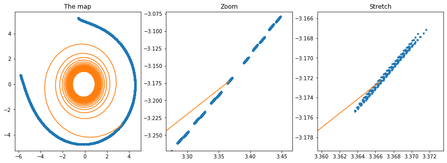
# Let us now visualize the Taylor map by creating a grid of perturbations on the initial conditions and
# evaluating the map for those values
Npoints = 20 # 10000 points
epsilon = 1e-3
grid = np.arange(-epsilon,epsilon,2*epsilon/Npoints)
nxf = [0] * len(grid)**4
nyf = [0] * len(grid)**4
i=0
import time
start_time = time.time()
for dr in grid:
    for dt in grid:
        for dvr in grid:
            for dvt in grid:
                nxf[i] = xf.evaluate({"dr":dr, "dt":dt, "dvr":dvr,"dvt":dvt})
                nyf[i] = yf.evaluate({"dr":dr, "dt":dt, "dvr":dvr,"dvt":dvt})
                i = i+1
print("--- %s seconds ---" % (time.time() - start_time))

--- 23.139215230941772 seconds ---

f, axarr = plt.subplots(1,3,figsize=(15,5))
# Normal plot of the final map
axarr[0].plot(nxf,nyf,'.')
axarr[0].plot(cx,cy)
axarr[0].set_title("The map")

# Zoomed plot of the final map (equal axis)
axarr[1].plot(nxf,nyf,'.')
axarr[1].plot(cx,cy)
axarr[1].set_xlim([cx[-1] - 0.1, cx[-1] +0.1])
axarr[1].set_ylim([cy[-1] - 0.1, cy[-1] +0.1])
axarr[1].set_title("Zoom")

# Zoomed plot of the final map (unequal axis)
axarr[2].plot(nxf,nyf,'.')
axarr[2].plot(cx,cy)
axarr[2].set_xlim([cx[-1] - 0.007, cx[-1] + 0.007])
axarr[2].set_ylim([cy[-1] - 0.007, cy[-1] + 0.007])
axarr[2].set_title("Stretch")
#axarr[1].set_xlim([cx[-1] - 0.1, cx[-1] + 0.1])
#axarr[1].set_ylim([cy[-1] - 0.1, cy[-1] + 0.1])

Text(0.5, 1.0, 'Stretch')

5.5. How much faster is now to evaluate the Map rather than perform a new numerical integration?

# First we profile the method evaluate (note that you need to call the method 4 times to get the full state)

%timeit xf.evaluate({"dr":epsilon, "dt":epsilon, "dvr":epsilon,"dvt":epsilon})

59.5 µs ± 4.74 µs per loop (mean ± std. dev. of 7 runs, 10000 loops each)

# Then we profile the Runge-Kutta 4 integrator

%%timeit
D.set_float_fmt('float64')
float_integration = de.OdeSystem(eom_kep_polar, y0=[it + epsilon for it in ic], dense_output=False, t=(0, 300.), dt=0.01, rtol=1e-10, atol=1e-10, constants=dict())

float_integration.set_method("RK45")
float_integration.integrate(eta=False)

422 ms ± 31.2 ms per loop (mean ± std. dev. of 7 runs, 1 loop each)

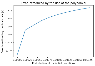
# It seems the speedup is 2-3 orders of magnitude, but did we loose precision?
# We plot the error in the final result as computed by the HOTM and by the Runge-Kutta
# as a function of the distance from the original initial conditions
out = []
pert = np.arange(0,2e-3,2*1e-4)
for epsilon in pert:
    res_map_xf = xf.evaluate({"dr":epsilon, "dt":epsilon, "dvr":epsilon,"dvt":epsilon})
    res_int = de.OdeSystem(eom_kep_polar, y0=[it + epsilon for it in ic], dense_output=False, t=(0, 300.), dt=0.01, rtol=1e-10, atol=1e-10, constants=dict())
    res_int.set_method("RK45")
    res_int.integrate()
    res_int_x = [it.y[0]*np.sin(it.y[2]) for it in res_int]
    res_int_xf = res_int_x[-1]
    out.append(np.abs(res_map_xf - res_int_xf))
plt.semilogy(pert,out)
plt.title("Error introduced by the use of the polynomial")
plt.xlabel("Perturbation of the initial conditions")
plt.ylabel("Error in estimating the final state (x)")

Text(0, 0.5, 'Error in estimating the final state (x)')